Same JSON Storage Problem, Different Database - What Postgres Does Differently
Background
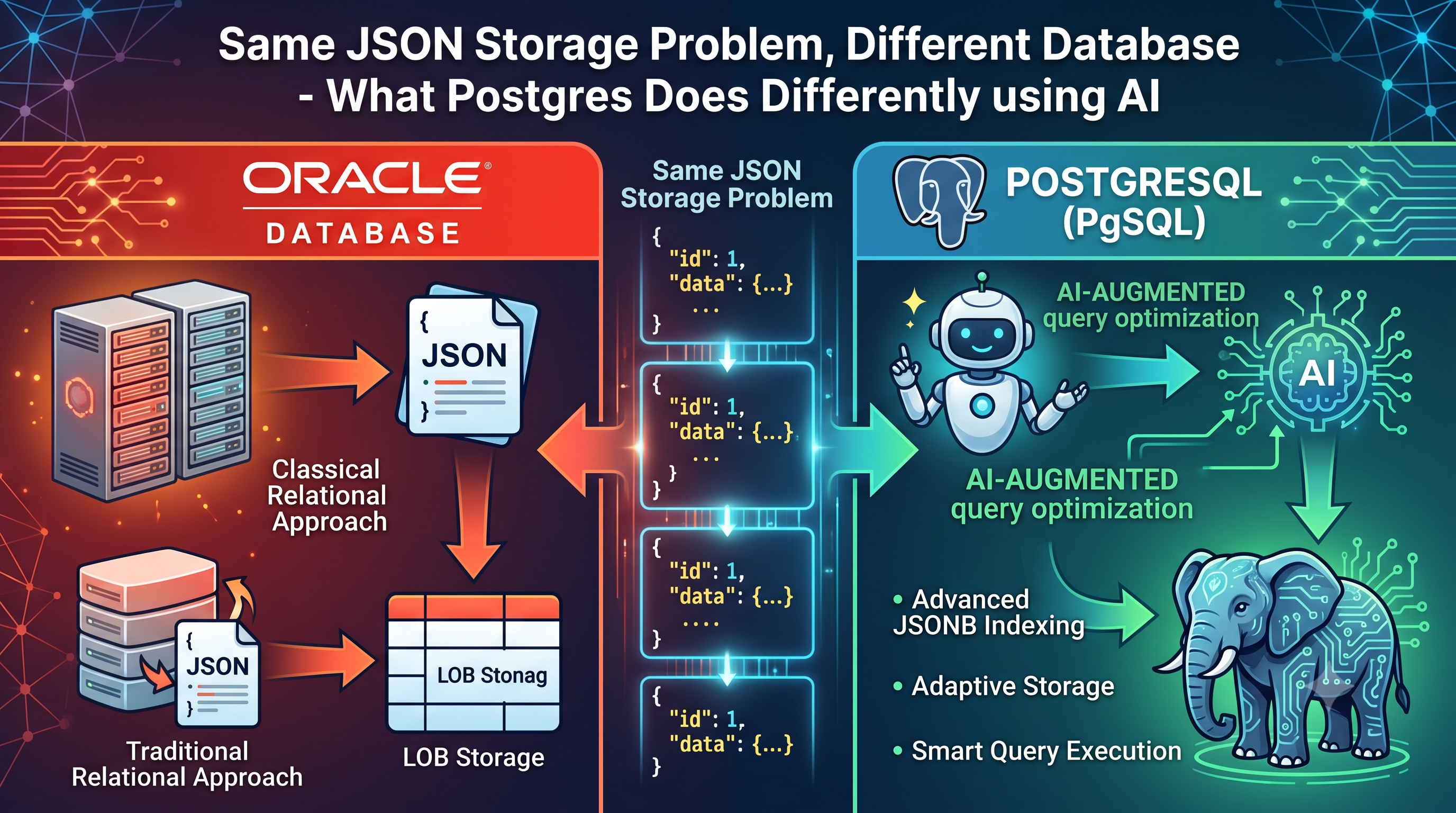
My earlier article on AI augmented Fintech post-mortem review walked through an Oracle JSON storage problem: a payment transaction table stored as JSON, a query that needed to filter on a nested field, and the chain of fixes - that the team eventually needed.
Out of curiosity - a reasonable question came out of that post: does Postgres have the same problem?
The honest answer is partly yes, partly no. Postgres stores JSON differently to Oracle, and it has indexing options for JSON data that Oracle's virtual column approach doesn't have a direct equivalent for. But the underlying lesson - that a flexible storage format which looks fine at low row counts can become a real query performance problem at scale - still applies. It just plays out differently.
To make this concrete rather than theoretical, I built a 3-million-row Postgres table with the same shape of payment data as the Oracle example - JSONB payload, nested merchant category, card network, risk signals - with realistic looking skewed distribution instead of uniform data, and ran real queries against it. Every plan and timing number in this post is captured directly from that table.
This post covers:
- The setup - the table, the data, why the skew matters
- The baseline query, unindexed, and what the plan shows
- The fix - and a planner behaviour that's worth understanding before you trust it
- A second slow pattern - what a reconciliation-style aggregation query reveals
- The prompt I used to walk through both plans systematically
1. The setup
The table:
1CREATE TABLE payment_transactions (
2    id              BIGSERIAL PRIMARY KEY,
3    transaction_id  UUID NOT NULL DEFAULT gen_random_uuid(),
4    created_at      TIMESTAMPTZ NOT NULL,
5    amount_minor    BIGINT NOT NULL,
6    currency        CHAR(3) NOT NULL,
7    status          VARCHAR(20) NOT NULL,
8    payload         JSONB NOT NULL
9);
payload carries everything payment-method-specific - merchant category, card network, risk score, settlement cycle - nested two and three levels deep, the same shape as the Oracle example:
 1{
 2  "paymentDetail": {
 3    "merchantInfo": { "category": "HEALTHCARE", "merchantId": "M2381" },
 4    "cardInfo": { "network": "VISA", "last4": "4821" }
 5  },
 6  "metadata": {
 7    "riskSignals": { "score": 12.4, "band": "LOW" },
 8    "channel": "MOBILE_APP"
 9  },
10  "settlement": { "cycle": "T+2", "settlementCurrency": "INR" }
11}
3 million rows, generated with deliberate skew rather than even distribution - because thats what you generally see in your production systems.
| Category | Row count | Share |
|---|---|---|
| FASHION | 1,123,030 | 37.4% |
| ELECTRONICS | 959,875 | 32.0% |
| GROCERY | 642,105 | 21.4% |
| TRAVEL | 219,829 | 7.3% |
| FOOD_DELIVERY | 48,608 | 1.6% |
| HEALTHCARE | 6,174 | 0.2% |
| EDUCATION | 371 | 0.01% |
| OTHER | 8 | ~0% |
This matters for everything that follows. A query filtering on FASHION and a query filtering on HEALTHCARE are touching the same column with the same index, but they're asking fundamentally different questions of the planner - one wants 1.1 million rows out of 3 million, the other wants 6,174. Within PostgreSQL a single index doesn't automatically mean a single plan.
2. The baseline query
A reconciliation-style lookup - find the 100 most recent successful HEALTHCARE transactions:
1SELECT transaction_id, amount_minor, created_at
2FROM payment_transactions
3WHERE payload->'paymentDetail'->'merchantInfo'->>'category' = 'HEALTHCARE'
4  AND status = 'SUCCESS'
5ORDER BY created_at DESC
6LIMIT 100;
No indexes exist yet on status or on anything inside payload. Here's the real
plan:
 1Limit  (cost=187192.93..187204.59 rows=100 width=32) (actual time=860.443..861.506 rows=100 loops=1)
 2  Buffers: shared hit=15536 read=142439
 3  ->  Gather Merge  (cost=187192.93..188211.50 rows=8730 width=32) (actual time=855.823..856.876 rows=100 loops=1)
 4        Workers Planned: 2
 5        Workers Launched: 2
 6        ->  Sort  (cost=186192.90..186203.81 rows=4365 width=32) (actual time=814.660..814.669 rows=77 loops=3)
 7              Sort Key: created_at DESC
 8              Sort Method: top-N heapsort  Memory: 36kB
 9              ->  Parallel Seq Scan on payment_transactions  (cost=0.00..186026.08 rows=4365 width=32) (actual time=8.417..812.072 rows=1439 loops=3)
10                    Filter: (((status)::text = 'SUCCESS'::text) AND ((((payload -> 'paymentDetail'::text) -> 'merchantInfo'::text) ->> 'category'::text) = 'HEALTHCARE'::text))
11                    Rows Removed by Filter: 998561
12Planning Time: 0.356 ms
13Execution Time: 879.233 ms
879ms. The plan is a parallel sequential scan - Postgres reads through the entire table across 2 worker processes, evaluating the JSON path expression on every single row, throwing away 998,561 rows per worker to find the 100 it actually wants.
Buffers: shared hit=15536 read=142439- roughly 158,000 8KB blocks touched.
Oracle post-mortem described the same fundamental problem!
3. The fix - and the part worth understanding before you trust it
Postgres has something Oracle's virtual-column workaround doesn't have a direct equivalent for: you can build an index directly on a JSON path expression, without adding a column to the table at all.
1CREATE INDEX idx_txn_category
2ON payment_transactions ((payload->'paymentDetail'->'merchantInfo'->>'category'));
3
4CREATE INDEX idx_txn_status ON payment_transactions (status);
5CREATE INDEX idx_txn_created_at ON payment_transactions (created_at DESC);
Re-running the exact same HEALTHCARE query:
 1Limit  (cost=18333.45..18333.70 rows=100 width=32) (actual time=49.780..49.798 rows=100 loops=1)
 2  Buffers: shared hit=392 read=5691
 3  ->  Sort  (cost=18333.45..18342.78 rows=3733 width=32) (actual time=49.778..49.788 rows=100 loops=1)
 4        Sort Method: top-N heapsort  Memory: 36kB
 5        ->  Bitmap Heap Scan on payment_transactions  (cost=61.11..18190.78 rows=3733 width=32) (actual time=2.149..48.480 rows=4317 loops=1)
 6              Recheck Cond: ((((payload -> 'paymentDetail'::text) -> 'merchantInfo'::text) ->> 'category'::text) = 'HEALTHCARE'::text)
 7              Filter: ((status)::text = 'SUCCESS'::text)
 8              Rows Removed by Filter: 1857
 9              Heap Blocks: exact=6072
10              ->  Bitmap Index Scan on idx_txn_category  (cost=0.00..60.18 rows=5300 width=0) (actual time=1.091..1.091 rows=6174 loops=1)
11                    Index Cond: ((((payload -> 'paymentDetail'::text) -> 'merchantInfo'::text) ->> 'category'::text) = 'HEALTHCARE'::text)
12Planning Time: 0.776 ms
13Execution Time: 49.913 ms
879ms down to 49.9ms - 17.6x improvement. Buffer touches down from 158,000 to about 6,000. One index, no application code changes, no schema migration.
Caveat - before treating this as a universal fix. Notice Recheck Cond in that plan - Postgres found candidate rows using the index, then had to go back to the actual table and recheck the condition. This happens because a B-tree index on a JSON path stores the extracted value, not a guarantee that matches it perfectly without re-verification at the row level for this query shape. It's not a sign of anything broken; it's simply not a free lookup the way a primary key index is.
Now let's understand what happens when the same query, same index, asks for a common category instead of a rare one:
1WHERE payload->'paymentDetail'->'merchantInfo'->>'category' = 'FASHION'
1Limit  (cost=0.43..94.97 rows=100 width=32) (actual time=0.080..2.862 rows=100 loops=1)
2  Buffers: shared hit=53 read=312
3  ->  Index Scan using idx_txn_created_at on payment_transactions  (cost=0.43..747013.93 rows=790125 width=32) (actual time=0.079..2.837 rows=100 loops=1)
4        Filter: (((status)::text = 'SUCCESS'::text) AND ((((payload -> 'paymentDetail'::text) -> 'merchantInfo'::text) ->> 'category'::text) = 'FASHION'::text))
5        Rows Removed by Filter: 262
6Planning Time: 0.096 ms
7Execution Time: 2.884 ms
2.9ms - even faster! But the plan isn't using
idx_txn_categoryat all. It's using thecreated_atindex instead, and just filtering FASHION rows out of whatever it finds along the way. The planner worked out that, no. of rows with FASHION at 37% of the table, the category index wouldn't actually narrow things down much, so scanning by date and filtering is cheaper than going through the category index.
That's what PostgreSQL planner is suppose to do - selecting different strategies for different SELECT criteria. It also means adding index doesn't necessarily guarantee faster queries. The same index can be the right tool for one filter value and not so relevant for another - on the exact same table and same query structure. Anyone tuning this in production needs to test across the actual range of values the application will query for, not just the one that happened to be slow in the bug report.
4. A second pattern - the reconciliation aggregation
A different kind of query that fintech systems run constantly - a settlement reconciliation report aggregating transaction volume by category and risk band over a rolling window:
 1SELECT
 2    payload->'paymentDetail'->'merchantInfo'->>'category' AS category,
 3    payload->'metadata'->'riskSignals'->>'band' AS risk_band,
 4    count(*) AS txn_count,
 5    sum(amount_minor) AS total_amount
 6FROM payment_transactions
 7WHERE status = 'SUCCESS'
 8  AND created_at > NOW() - INTERVAL '7 days'
 9GROUP BY 1, 2
10ORDER BY total_amount DESC;
690ms, even with the indexes from the previous section already in place:
 1Sort  (cost=187239.82..187443.99 rows=81665 width=104) (actual time=670.688..670.691 rows=21 loops=1)
 2  Buffers: shared hit=397 read=81014 written=201, temp read=347 written=348
 3  ->  GroupAggregate  (cost=172840.91..176107.51 rows=81665 width=104) (actual time=652.672..670.640 rows=21 loops=1)
 4        ->  Sort  (cost=172840.91..173045.07 rows=81665 width=72) (actual time=652.620..661.661 rows=81628 loops=1)
 5              Sort Method: external merge  Disk: 2776kB
 6              ->  Bitmap Heap Scan on payment_transactions  (cost=25205.79..162825.10 rows=81665 width=72) (actual time=152.416..621.248 rows=81628 loops=1)
 7                    Recheck Cond: ((created_at > (now() - '7 days'::interval)) AND ((status)::text = 'SUCCESS'::text))
 8                    Rows Removed by Index Recheck: 613652
 9                    Heap Blocks: exact=45866 lossy=33446
10                    ->  BitmapAnd  (cost=25205.79..25205.79 rows=81665 width=0)
11                          ->  Bitmap Index Scan on idx_txn_created_at (actual rows=116781 loops=1)
12                          ->  Bitmap Index Scan on idx_txn_status (actual rows=2099997 loops=1)
13Execution Time: 690.219 ms
Two things stand out here that the HEALTHCARE example didn't show.
First:
Sort Method: external merge Disk: 2776kB. The sort needed for the aggregation didn't fit in memory and spilled to disk. That's controlled bywork_mem, and it's worth checking before assuming the query itself is the problem.
Second:
Heap Blocks: exact=45866 lossy=33446. "Lossy" means Postgres ran out of room in its bitmap to track individual rows precisely and had to fall back to tracking whole pages instead - meaning it then had to recheck every row on those pages individually, which is whereRows Removed by Index Recheck: 613652comes from. That too is controlled bywork_mem. Status alone matches 2.1 million rows (SUCCESS is 90% of the table) - combining it with the date filter viaBitmapAndstill leaves a large enough candidate set that the bitmap representation runs out of precision.
Neither of these is something a single CREATE INDEX statement fixes. This is the kind of query where the actual lever is a memory setting, not an index.
5. The prompt that walks through this systematically
Reading one EXPLAIN ANALYZE output by hand is manageable. Reading four of them, cross-referencing buffer counts, recheck conditions, and selectivity differences between runs, and knowing whether the right fix is an index or a memory setting - that's the part worth turning into a repeatable process rather than redoing the reasoning from scratch each time.
The prompt I used asks for five specific things:
- Walk the actual cost and timing numbers in the plan rather than describing the query in general terms
- Identify whether the bottleneck is a missing index, a planner selectivity decision, or a memory-driven spill
- Explain anything unusual in the plan output specifically (Recheck Cond, lossy blocks, external merge)
- State what would happen if the same query ran against a different value with different selectivity
- Propose a specific, testable next step rather than a generic "add an index" response.
The first pass at this, run against the HEALTHCARE plan alone, gave a reasonable explanation of the speed-up but didn't flag the Recheck Cond line at all - it just ignored this flag initially. It only responded with proper explanation when asked specifically what "Recheck Cond" means and why it's there.
The same approach against the reconciliation query did better on its own - work_mem and the disk spill were highlighted without prompting. But it had no way of knowing what work_mem was actually set to in this environment, or whether raising it was safe given everything else running on the same instance.
The full prompt, plus both worked examples with the real plan output above, are in the GitHub repo.
Conclusion
The Oracle post-mortem from previous week and this Postgres example are not the same problem with the same fix. Oracle's virtual columns introduce a real write-side cost - every insert and update re-evaluates the virtual column expression. Postgres's expression index doesn't have that exact failure mode, but it has its own nuance - the same index can produce a completely different plan depending on how selective the filter value is.
What's consistent across both databases is the underlying lesson. A storage format that looks flexible and harmless at low row counts can hide real query cost that only shows up at scale - and the only way to know which fix would actually work is to read the real plan, and not assume from the table schema what the database is doing underneath it.
The full prompt used for this analysis is available in my se-ai-templates repository on GitHub.
comments powered by Disqus